Latent Profile Analysis (LPA) and related mixture models identify hidden subgroups in your data. Instead of assuming everyone in your sample comes from one population, LPA discovers distinct profiles — groups of people who share similar patterns of characteristics. This is essential for person-centered research in psychology, education, and social science.
Prerequisites
Basic understanding of means, standard deviations, and regression. Familiarity with the concept of probability distributions is helpful but not required. We build up from simple clustering to model-based classification step by step.
Software
R with tidyLPA and mclust packages for mixture models; Mplus is the gold standard for latent variable models in social science. Python alternatives include scikit-learn's GaussianMixture. All examples provided in R.
Part 1 · Slide 1
Variable-Centered vs. Person-Centered
V
Variable-Centered
Focus: Relationships among variables. Assumption: Single homogeneous population. Examples: Regression, SEM, ANOVA, CFA. i.e.: "Does higher intrinsic motivation predict better achievement?"
P
Person-Centered
Focus: Identifying subgroups of individuals. Assumption: Heterogeneous — distinct latent subgroups exist. Examples: LPA, LCA, Cluster Analysis. i.e.: "What types of motivation patterns exist among students?"
The mean can mask meaningful heterogeneity — person-centered methods reveal hidden diversity.
Part 1 · Slide 2
Person-Centered Analytical Methods
Cluster Analysis
Distance-based grouping (e.g., K-means)
No underlying statistical model
No formal test for optimal clusters
Hard assignment only
Today's Focus
LPA
Continuous indicators
Model-based (Finite Mixture Model)
Statistical fit indices for class enumeration
Probabilistic assignment
LCA
Categorical indicators
Same framework as LPA
Item response probabilities instead of means
Probabilistic assignment
Part 1 · Slide 3
How LPA Works: Mixture Models
LPA is built on a Finite Mixture Model: observed data is a mixture of K normal distributions, each representing a hidden subgroup. Using the EM algorithm, LPA infers how many subgroups exist, the mean and variance of each on each indicator, and each person's probability of belonging to each subgroup.
Overlapping Gaussians
Three profiles (red, gold, tea) overlap. Each person's scores are drawn from one of these distributions.
Part 1 · Slide 4
Probabilistic Classification
Unlike hard clustering (e.g., k-means), LPA gives each individual a probability of belonging to each class. Classification uses the highest posterior probability, but uncertainty is preserved.
i.e.: A student has 82% probability of belonging to Profile 1, 13% to Profile 2, 5% to Profile 3. We assign them to Profile 1, but acknowledge 18% uncertainty. This is softer than hard clustering which forces 100% membership.
Part 1 · Slide 5
Choosing the Right Number of Profiles
BIC
Bayesian Information Criterion
Lower values indicate better fit. Look for the "elbow" where the decrease slows down. Penalizes model complexity.
BLRT
Bootstrapped Likelihood Ratio Test
Most accurate test across conditions. Significant p-value (< .05) means k classes fit better than k-1. Keep adding classes until p ≥ .05.
ENT
Classification Quality
Ranges 0–1. Values > .80 indicate clear class separation. Close to 1 = clean assignment. But DO NOT use it for class selection alone.
Decision Rule: When indices disagree, prioritize BLRT + BIC, combined with theoretical interpretability. Class sizes should be at least 5–8% of your sample to avoid unstable profiles.
Part 1 · Slide 6
LPA Workflow: 5 Steps
01
Theory & Indicators
Select indicators from theoretical framework
02
Fit 1 to K Models
Incrementally increase class number
03
Compare Fit Indices
BIC, BLRT, entropy
04
Interpret Profiles
Read profile plot, name classes
05
Validate
Covariates & outcomes (three-step)
Practical Tips.Sample size: N ≥ 300–500 (Nylund-Gibson & Choi, 2018). Random starts: ≥ 500 to avoid local solutions. Smallest class: ≥ 5–8% of sample. Entropy: > .80 indicates good classification — but do NOT use it to select K.
Part 2 · Slide 1
Article Example
Wang, C. K. J., Liu, W. C., Nie, Y., et al. (2017). Latent profile analysis of students' motivation and outcomes in mathematics: An organismic integration theory perspective. Heliyon, 3(6), e00308. Open Access
Core question: Are there distinct subgroups of students characterized by unique combinations of motivations — and do these profiles predict different academic outcomes?
RQ
Theoretical Framework
Organismic Integration Theory (OIT), a sub-theory of Self-Determination Theory, posits that motivation is not "high vs. low" but a continuum — from external regulation to intrinsic motivation. Each student has a simultaneous score on all four types, creating a unique combination pattern. Variable-centered methods miss this; LPA captures it.
Part 2 · Slide 2
Article Example: Study Design
01
Sample
N = 1,151 secondary students (age 13–17, M = 14.69) from 5 schools in Singapore. 679 males, 444 females, 28 unreported.
At least 4 distinct profiles will emerge based on OIT motivation types.
H2
Hypothesis 2
More autonomous profiles → higher effort, value, competence, and extra time on math.
Part 2 · Slide 3
Step 1: Model Comparison & Class Enumeration
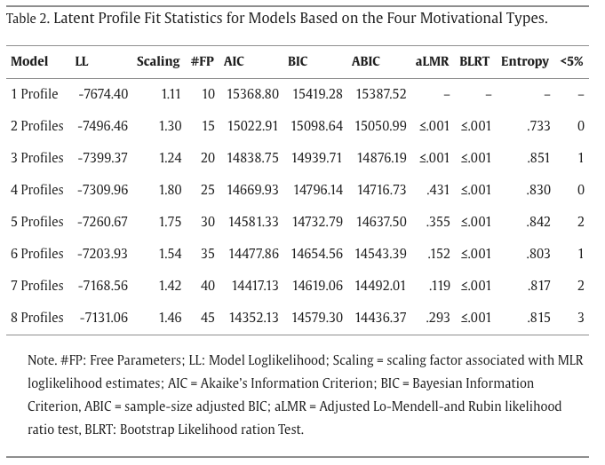
Table 2. Latent profile fit statistics for models with 1–8 profiles based on the four motivational types.
Decision Rules (Nylund et al., 2007; Nylund-Gibson & Choi, 2018). BIC: Lower is better — look for the "elbow" where decline slows. BLRT: Most accurate across all conditions — significant p means K > K−1. aLMR: Adjusted Lo-Mendell-Rubin test — non-significant p suggests current K is sufficient. When indices disagree: Prioritize BIC + BLRT, combined with theoretical interpretability and class size. Here, the 4-profile solution was selected: the aLMR became non-significant beyond 4 profiles, fit improvements were marginal, and each profile was theoretically interpretable.
BLRT: Tests whether k classes fit significantly better than k-1. If p < .05, you should add another class. Keep adding until the test says "no significant improvement."
Result: The 4-profile solution was selected. The aLMR p-value became non-significant (p = .12) beyond 4 profiles, indicating that adding a 5th profile did not significantly improve the model. All other indices agreed: BIC showed an elbow at k=4, and each of the four profiles was theoretically meaningful and interpretable.
Part 2 · Slide 4
Step 2: Interpreting the Profile Plot
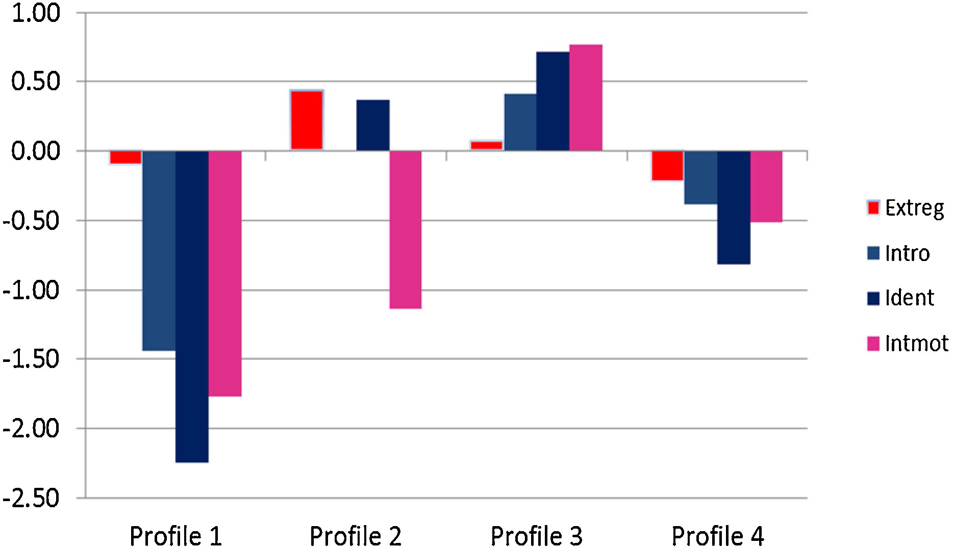
Figure 1. Four motivation profiles across four SDT indicators (Extreg = External Regulation, Intro = Introjected Regulation, Ident = Identified Regulation, Intmot = Intrinsic Motivation).
5.8%
Low Motivation
Near-average external regulation but very low introjected, identified, and intrinsic motivation (n = 67)
Near 5% threshold — may be unstable with smaller samples
10.2%
Externally Driven
High external & identified regulation, but very low intrinsic motivation — regulated by external demands (n = 118)
50.7%
Autonomous
High identified regulation & intrinsic motivation — the most self-determined and largest group (n = 584)
33.2%
Moderate
Low identified regulation & intrinsic motivation with moderate external and introjected regulation (n = 382)
Reading Profile Plots. Focus on the shape of the line (the pattern across indicators), not just absolute levels. Name each profile based on its most distinctive features.
Part 2 · Slide 5
Step 3: Outcome Validation
Do the profiles differ on meaningful academic outcomes?
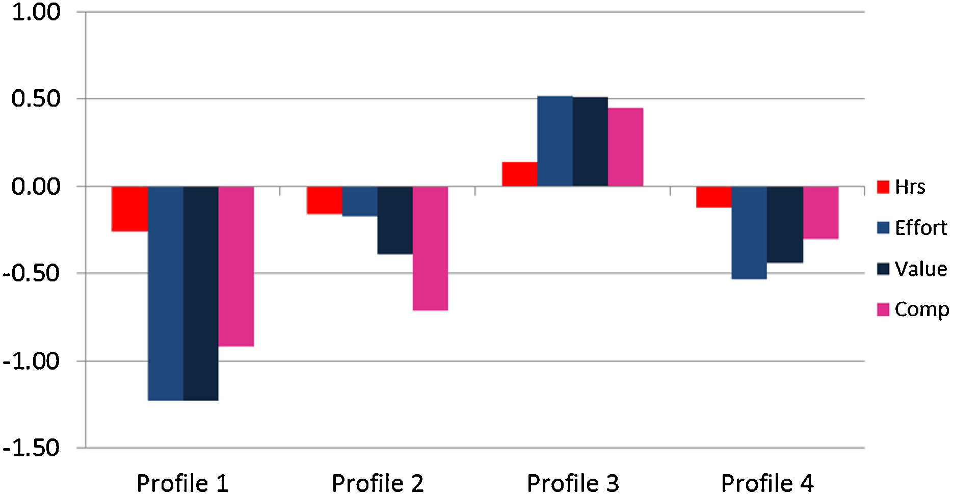
Figure 2. Outcome differences across four profiles (Hrs = Math Study Time, Effort = Self-Reported Effort, Value = Task Value, Comp = Perceived Competence).
Autonomous Advantage
The Autonomous profile (P3) consistently outperformed all other groups across every outcome: effort (3 > 2 > 4 > 1), task value (3 > 2 = 4 > 1), perceived competence (3 > 4 > 2 = 1), and math study hours (3 > 4 = 2 = 1). High autonomous motivation led to the most adaptive outcomes.
Effort Is Graded by Self-Determination
Effort showed a clear gradient across profiles: P3 > P2 > P4 > P1. Notably, the Externally Driven group (P2) reported higher effort than the Moderate group (P4), suggesting external pressure can sustain effort — but the Autonomous group's effort still surpassed all others.
Competence Requires Intrinsic Interest
The Externally Driven profile (P2) showed no advantage in perceived competence over the Low Motivation group (P1), despite P2's higher external and identified regulation (2 = 1). In contrast, even the Moderate group (P4) outperformed P2 in competence, suggesting that intrinsic interest — not external pressure — is essential for building academic confidence.